Introduction
This multinational dataset from Kaggle contains transactions from a UK-based online retailer between December 1, 2010 and December 9, 2011. Its size makes it well suited to customer segmentation with machine-learning techniques such as K-Means.
The workflow is straightforward: clean and explore the data, create a rule-based segmentation with the RFM model, and then use K-Means clustering for an unsupervised second view. The two methods can then be compared against each other.
Data Sources
https://www.kaggle.com/yasserh/customer-segmentation-dataset
https://archive.ics.uci.edu/ml/datasets/online+retail
Dataset
The dataset contains 540,545 rows and eight columns:
| Field | Description |
|---|---|
| InvoiceNo | A six-digit invoice number assigned to each transaction. A value beginning with C indicates a cancellation. |
| StockCode | Product code |
| Description | Product name |
| Quantity | Quantity purchased |
| InvoiceDate | Invoice date and time |
| UnitPrice | Unit price in pounds sterling |
| CustomerID | Customer identifier |
| Country | Country |
Objectives
- Preprocess and clean the dataset, then perform exploratory data analysis
- Segment customers by similarity and build both an RFM profile and a K-Means clustering model
- Tune the model and compare relevant evaluation metrics
Importing Libraries
1
2
3
4
5
6
7
import pandas as pd
import numpy as np
from pyecharts.charts import *
import pyecharts.options as opts

import warnings
warnings.filterwarnings('ignore')
Data Preprocessing
1
2
3
4
5
6
7
8
9
10
11
12
13
14
15
16
17
18
19
20
## Read the data
df = pd.read_excel('D:/**/Online Retail.xlsx')

## Remove rows without a customer ID
df.dropna(subset=['CustomerID'], inplace=True)

## Convert timestamps to strings
df['InvoiceDate'] = df['InvoiceDate'].map(lambda x: str(x))

## Normalize country names
df.replace({
    'EIRE': 'Ireland',
    'USA': 'United States',
    'RSA': 'South Africa',
    'Czech Republic': 'Czech',
    'Channel Islands': 'United Kingdom'
}, inplace=True)

## Calculate line-item value
df['Amount'] = df['Quantity'] * df['UnitPrice']
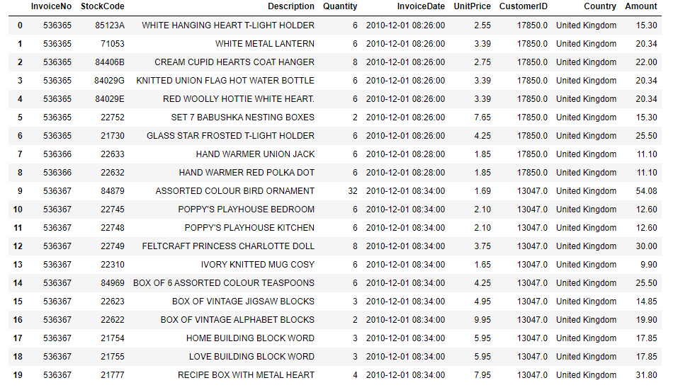
Preview of the Processed Data
1
df.head(20)
Exploratory Data Analysis
1
2
3
4
5
6
7
8
9
10
11
## Classify transaction status
df['InvoiceNo'] = df['InvoiceNo'].astype(str)
df['Transaction status'] = df['InvoiceNo'].map(
    lambda x: '0' if x.startswith('C') else '1'
)

## Visualize transaction status
label = ['Completed', 'Cancelled']
value = df['Transaction status'].value_counts().values.tolist()

## Additional plotting code omitted for brevity
Findings
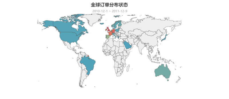
- The United Kingdom has the largest number of orders. Most transactions are concentrated in Europe around the UK, although the dataset also includes orders from North America, South America, and Australia.
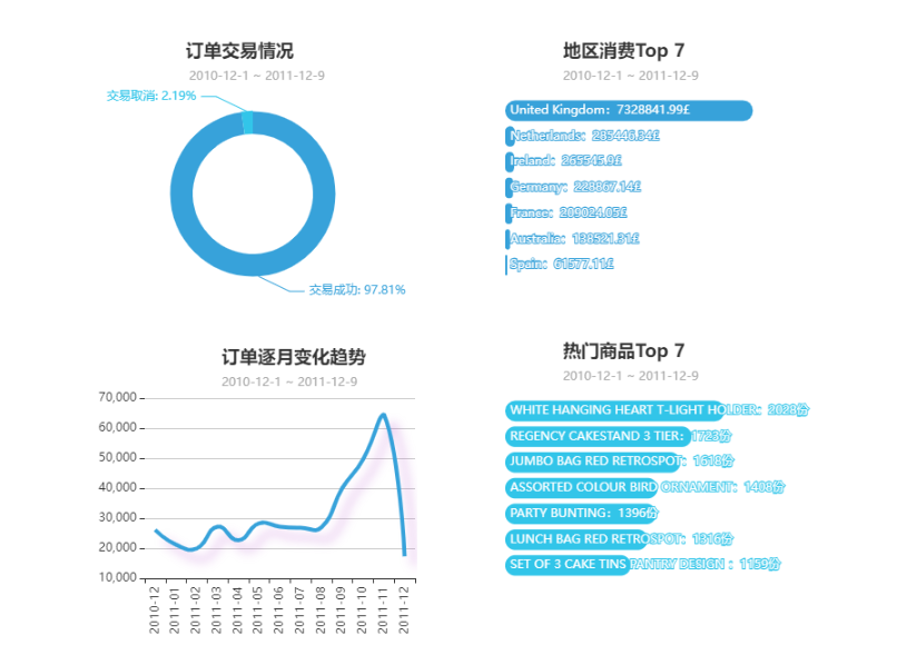
- Cancellations and returns are limited. Completed transactions account for 97.81% of all orders; cancellations or returns account for 2.19%.
- November 2011 is the peak month. Order volume rose noticeably from August through November 2011.
- Most popular product. The top-selling item is
WHITE HANGING HEART T-LIGHT HOLDER.
Customer Segmentation with RFM
RFM describes customer value across three dimensions: R (Recency, days since the most recent purchase), F (Frequency, purchase frequency), and M (Monetary, total spend). The following code bins and scores each measure, then splits the scores into high and low groups around their mean values.
1
2
3
4
5
6
7
8
9
10
11
12
13
14
15
16
17
18
19
20
21
22
23
24
25
## Calculate total spend for each customer
df_total = pd.DataFrame(
    df.groupby('CustomerID')['Amount'].sum()
).reset_index()
df_total.columns = ['CustomerID', 'Total_Amount']
df_total['Total_Amount'] = df_total['Total_Amount'].map(
    lambda x: round(x, 2)
)

## Extract date and time from each order
df['InvoiceDate_ymd'] = df['InvoiceDate'].map(lambda x: x.split(' ')[0])
df['InvoiceDate_hms'] = df['InvoiceDate'].map(lambda x: x.split(' ')[1])

## RFM scoring: step 1
## A smaller score represents a higher tier
df_rfm['R_level'] = pd.cut(df_rfm['R'], bins=[0,65,130,195,260,325,390], labels=[1,2,3,4,5,6], right=False)
df_rfm['F_level'] = pd.cut(df_rfm['F'], bins=[0,10,20,50,100,175,250], labels=[6,5,4,3,2,1], right=False)
df_rfm['M_level'] = pd.cut(df_rfm['M'], bins=[0,28,280,2800,28000,145000,285000], labels=[6,5,4,3,2,1], right=False)

## RFM scoring: step 2
df_rfm['R_level'] = df_rfm['R_level'].map(lambda x: 'High' if x < df_rfm['R_level'].astype(int).mean() else 'Low')
df_rfm['F_level'] = df_rfm['F_level'].map(lambda x: 'High' if x < df_rfm['F_level'].astype(int).mean() else 'Low')
df_rfm['M_level'] = df_rfm['M_level'].map(lambda x: 'High' if x < df_rfm['M_level'].astype(int).mean() else 'Low')

## Additional code omitted for brevity
Finding
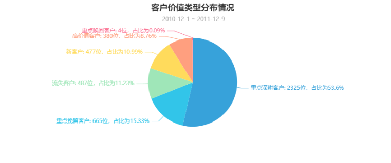
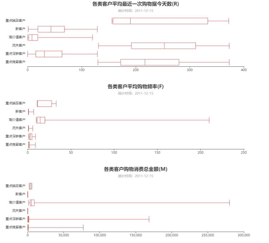
The rule-based RFM segmentation classifies 53.6% as high-potential customers, 15.33% as priority-retention customers, and only 0.09% as priority win-back customers.
K-Means Cluster Analysis
RFM uses manually selected thresholds. K-Means provides an unsupervised alternative that reveals how the observations naturally group together.
1
2
3
4
5
6
7
8
9
10
11
12
13
14
15
16
17
18
19
20
from sklearn.preprocessing import MinMaxScaler
from sklearn.cluster import KMeans
from sklearn.metrics import silhouette_score

K = range(1, 10)
meandistortions = []
for k in K:
    kmeans = KMeans(n_clusters=k)
    kmeans.fit(data_scaled)
    meandistortions.append(
        sum(np.min(cdist(data_scaled, kmeans.cluster_centers_, 'euclidean'), axis=1))
        / data_scaled.shape[0]
    )
plt.plot(K, meandistortions, marker='o')
plt.xlabel('K')
plt.ylabel('Average distortion')
plt.title('Selecting K with the Elbow Method')
plt.show()

# Additional code omitted for brevity
Choosing K
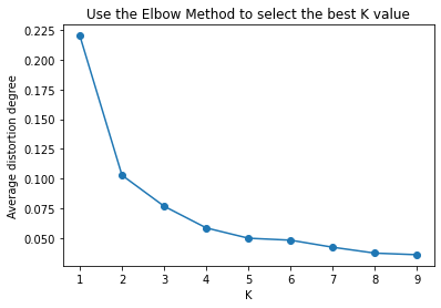
The average distortion begins to flatten at K=4. Increasing K beyond that point brings little improvement, so I use four clusters.
Cluster Visualization
1
2
3
4
5
6
7
8
Kmeans = KMeans(n_clusters=4, max_iter=50)
Kmeans.fit(data_scaled)
cluster_labels_k = Kmeans.labels_
df_rfm = df_rfm.reset_index()
cluster_labels = pd.DataFrame(cluster_labels_k, columns=['clusters'])
res = pd.concat((df_rfm, cluster_labels), axis=1)

## Additional code omitted for brevity
Cluster Profiles
Cluster 1
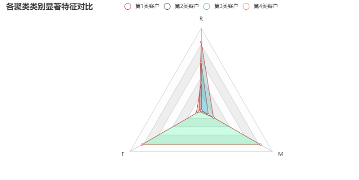
These customers purchased a long time ago, have zero recent purchase frequency, and spent relatively little. They are typical churned customers.
Cluster 2
These customers purchased very recently, buy frequently, and spend heavily. They are typical high-value customers.
Cluster 3
These customers resemble Cluster 1, but still have some—though limited—purchase activity. They are priority win-back customers.
Cluster 4
These customers purchased recently but have low frequency and zero recorded spend. They may be new customers.
Summary
The exploratory analysis, RFM segmentation, and K-Means clustering point in the same direction: high-value and high-potential customers contribute most of the revenue but represent a limited share of the customer base, while many customers are inactive or low-frequency. Operationally, the business should focus on retaining high-value customers, reactivating churned customers, and building a conversion path for new customers. That is the practical value of granular customer segmentation.
-
Previous
How to Speed Up pip Package Downloads -
Next
For $2 a Month, AI Translates the X Creators I Follow and Delivers Their Posts to Feishu